My Summer at LEAP

Finding Equations with Machine Learning to Make Climate Models More Accurate

The Earth’s climate is a complicated system. To make sense of it, and to predict the impact of our actions on our climate, scientists need accurate climate models, called Earth System Models (ESMs). ESMs help scientists make forecasts by simulating interactions between the atmosphere, biosphere, cryosphere, land, and oceans. However, these massive computer simulations are expensive to run, often requiring months of supercomputer time. Because of this, they are run at a coarse resolution, chopping up the Earth into \(100 \times 100\) kilometer grid cells, and reporting key measurements such as temperature and humidity for each cell. As each grid cell is larger than the entire state of Rhode Island, this resolution is often far too coarse to properly model, or “resolve”, the effects of small scale events, such as a minor thunderstorm and its subsequent flash flooding. Although these events may be on the order of a few meters or kilometers, they can have drastic impacts on the accuracy of long term predictions. This is because our climate is a chaotic system, and small initial changes can result in large differences over time – a phenomenon commonly referred to as the butterfly effect.

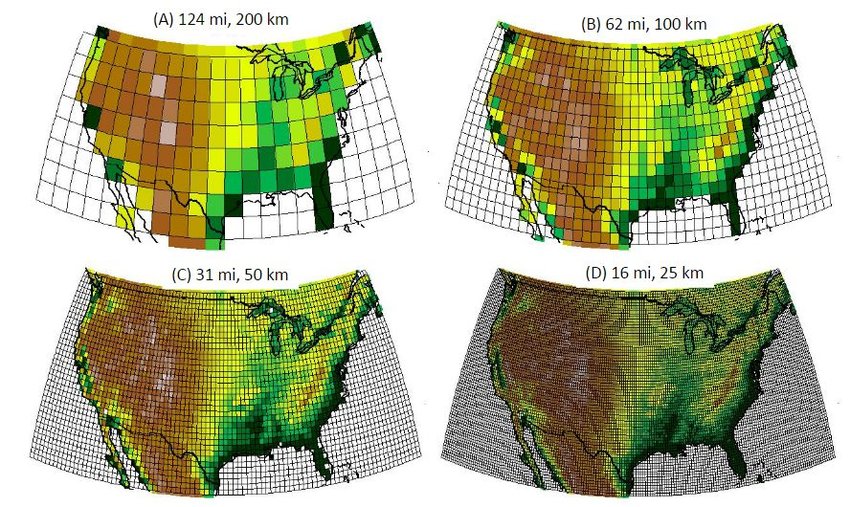
Figure 1: Comparison of different grid resolutions on a map of the contiguous United States [1].

Machine learning (ML) and artificial intelligence (AI) constitute a set of algorithms that learn patterns through data, and have become ubiquitous in our society through technologies like ChatGPT, self-driving cars, and targeted advertising. Due to their ability to efficiently ingest large volumes of data, ML methods present themselves as strong candidates for improving climate predictions by modeling these critical, small scale processes. A key concern is the black-box nature of many ML algorithms: it is often difficult to understand how these complex models arrive at their conclusions. For a prediction to be meaningful, the model must also be interpretable; scientists need to trust and understand the results to assign physical significance to the model’s outputs.

My name is Antony Sikorski, and I am a 2024 LEAP Momentum Fellow with a research focus in interpretable machine learning for climate models. I work on a project led by Dr. Sara Shamekh, where our group aims to understand vertical turbulent fluxes in the planetary boundary layer (PBL), which represent a major source of uncertainty for today’s climate models [2]. The PBL is the lowest part of the atmosphere and is most affected by Earth’s surface. Fog, pollution, and almost all human activity happen within the PBL. When we check our weather apps, the temperature and humidity forecasts describe conditions within the PBL. When we talk about the “vertical turbulent flux” of heat and moisture, we are referring to the transfer of these quantities between the Earth’s surface, and the atmosphere. This transfer is an example of a process that occurs on a small scale, yet can greatly impact long term predictions if not accounted for.

Figure 2: The divide between the PBL and the rest of the atmosphere displayed by the smog in Los Angeles, CA [3].

Scientists build these unresolved processes into ESMs by developing simplified representations of them, called parametrizations. These parameterizations are typically equations that use existing variables from the model and satisfy theoretical physics constraints. Putting it all together, our goal is to develop equations that make physical sense and accurately represent the transfer of key quantities, like heat, from the surface of the Earth to the atmosphere.

Before applying machine learning to these kinds of problems, scientists relied on a tedious combination of trial-and-error, intuition, and physics to come up with parametrizations. When ML algorithms were initially applied to the task, analytical equations were traded for predictive performance. Flexible models like neural networks were used to capture complex patterns in the data due to their large number of parameters and inherently nonlinear nature. Despite excellent accuracy, scientists remain cautious about trusting them because there is no neat way to extract the function “learned” by the neural net.

This summer, we’ve been working with a technique called symbolic regression, a machine learning task that aims to combine both accuracy and interpretability. After feeding in the inputs and outputs of our data, the symbolic regression algorithm provides us with a mathematical equation that it believes to be a good fit. It does this by learning to combine common operators \( (+, -, \times, /, ^\wedge ) \), coefficients \( (1,2,3) \), and primitive functions \( (sin(x), e^x) \). By using an algorithm inspired by the process of natural selection, symbolic regression compares its generated equations, and iteratively modifies and optimizes them until it reaches one that fits the data well enough.

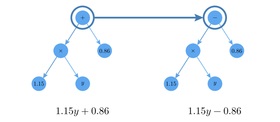
Figure 3: A visual example of generated equations being modified via a simple sign-change operation within the symbolic regression algorithm (adapted from [4]).

In order to develop these parametrizations, we need informative data. To create such data, we run high resolution simulations of the PBL, which are on the order of a few meters. This finer resolution allows us to see the small scale eddies and turbulent movements that vertically transfer key quantities like heat. After wrangling this data into a properly usable form, we spent most of our summer tuning our symbolic regression software, using our knowledge of statistics and physics to see how well these equations fit, and considering whether they make sense or not.

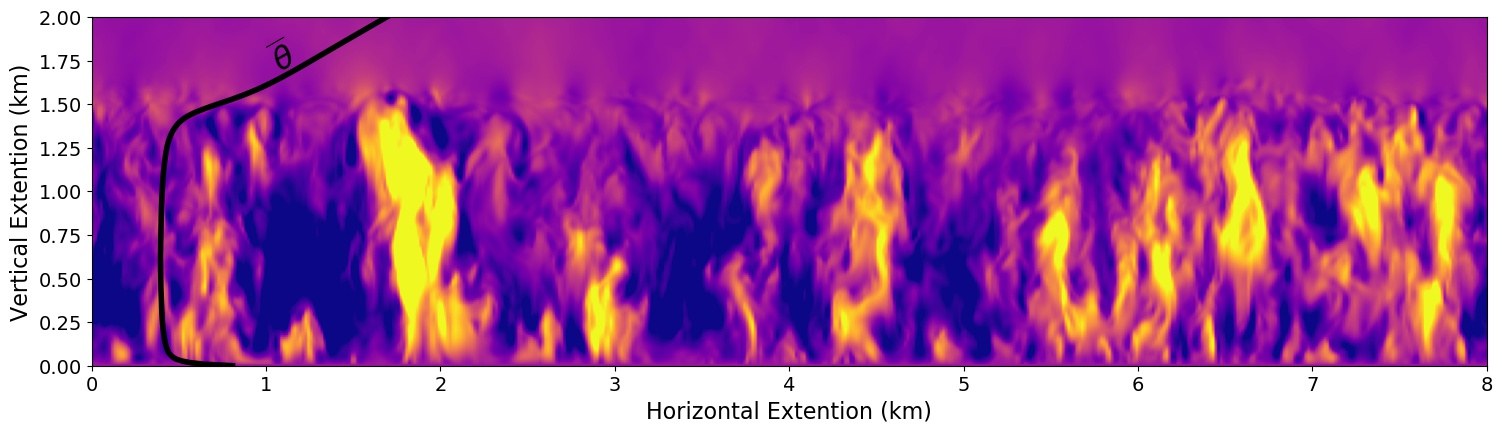
Figure 4: A slice of our high resolution, simulated data, where lighter colors represent a higher vertical velocity of air. Many small-scale, turbulent processes are shown, ranging from a few meters to a few km in size. The vertical profile of the average temperature (\(\overline{\theta}\)) is also imposed on the plot. (Courtesy of S. Shamekh)

So far, we have a number of exciting results, including the successful rediscovery of several equations that (mostly) agree with other recent parameterizations established by researchers. We believe the discrepancies are due to some dependence on other factors that are not being accounted for in prior studies, but teasing out the exact answer remains a work in progress. One reason uncovering these dependence relationships is difficult is the inherent randomness of the symbolic regression algorithm. There is no guarantee that the algorithm will converge or find the right equation, and as the number of candidate variables for the final parametrization increases, so does the difficulty of the search.

Figure 5: Presenting results to the NY Climate Exchange (Courtesy of A. Sikorski)

Machine learning algorithms have proven to be a tool with potential for transformative impact in numerous fields. While improving the accuracy of climate models is paramount, doing so with interpretable equations that scientists can trust and understand is arguably more important. Learning about, and implementing these equation-discovery algorithms to rediscover and expand our current understanding of the atmosphere has proven to be nothing short of rewarding.

References

1. Skees, Jerry R. “Financial Disaster Risk Management to Facilitate Recovery Lending” (2016)
2. Shamekh, Sara, and Pierre Gentine. “Learning atmospheric boundary layer turbulence.” Authorea Preprints (2023).
3. Britannica. (n.d.). Smog. Retrieved from https://www.britannica.com/science/smog
4. Cranmer, Miles. “Interpretable machine learning for science with PySR and SymbolicRegression. jl.” arXiv preprint arXiv:2305.01582 (2023).